Welcome to STARKFX.com page on Using the Discrete Fourier Transform
On this page, I will show my matlab code for taking advantage of the DFT (discrete fourier transform) to process images, allowing me to choose a given set of spatial frequencies to allow in reconstructing an image.
Image Basics
Looking at an Image as a 2D Array of Pixels, we can use a coordinate system to display the Brightness value for a given pixel
So, let's read in an image file:
If we display this image, we see it is in color:

So, we will change it to grayscale using a matlab provided function that uses the RGB values in the image array to determine a grayscale value to replace it. That way we have a single 2D array rather than 3 such 2D arrays representing the red (R), green (G) and blue (B) component values that make up most jpeg images.
We will then do a little conditioning to put the values for the pixels all in the range from 0 to 1:
Now we can see it is a grayscale image:
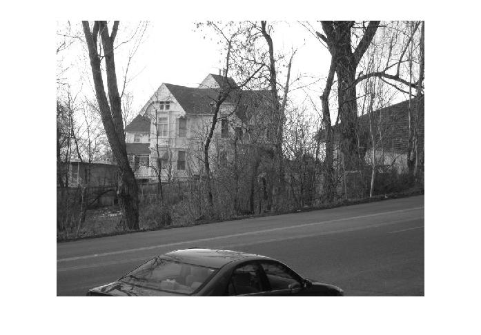
Take the 2D discrete fourier transform:
Split out magnitude and phase:
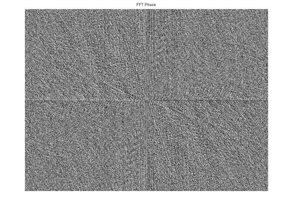
This splitting process works because the result of the fft2 function is a complex array. The magnitude given by the absolute value of this array is the magnitude of the spatial frequency component represented by that location in the array. The angle gives the phase for that spatial frequency component. (Phase actually turns out to be the more important value for reconstructing an image since it tells the phases relative to each other for all of the spatial frequency components so that when they add together, we get the particular light and dark pattern that makes up our image.
Now, we are going to apply a little trick in order to visualize our FFT results a bit more intuitively. The spatial frequencies represented by the FFT in a 2D array span from f=[-N/2,-(N-1)/2, -(N-2)/2....0.....(N-2)/2, (N-1)/2]*Fs/N where Fs is the sampling frequency (1 sample per pixel) and N is the number of pixels in that dimension. So as in our example with 964 pixels in the x direction and 686 pixels in the y direction we get frequencies from negative 1/2 cycle per pixel to a positive 1/2 cycle per pixel. Negative and positive frequencies really represent the same frequencies so we don't need to keep both and you will see that the fft results are always symmetric with respect to the negative and positvie frequencies. Resolution in frequency space, or the step size in spatial frequency represented as we move from one point in the array to an adjacent point in the array is 1/N or, in our case, just looking at the x dimension, 1/964 cycle per pixel. These frequencies are nicely represented in an array with the zero frequency component (average level of the whole image) in the center of the array with increasing frequencies stepping at a rate of 1/964th cycle per pixel as we step in the x direction and 1/686th cycle per pixel as we step in the y direction away from the center of the image.
But, that is not exacty what we get from the output of the fft2 function. Instead, we get an array with the zero frequency components in the corners of the array and the highest frequency at the center (1/2 cycle per pixel in either direction). So, we use a function that simply, directly swaps our quadrants such that the frequency of one half cycle per pixel is at the edges of the array, while the zero component is at the center. This is really just for our benefit in displaying the magnitude and phase information. The function that accomplishes this switch is:
So, let's look at the phase information in an array form:
Notice that the values of the phase run from -pi to pi.
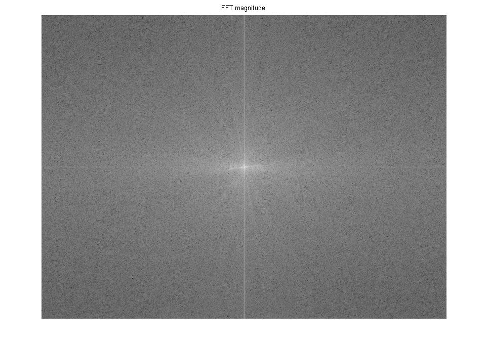
We are also going to use a little trick to enhance the contrast in displaying the magnitude at each spatial frequency component. We will take the log of the value so that the huge component magnitude at very low spatial frequencies does not completely drown out the high spatial frequency components in our display of the magnitudes at the various spatial frequencies.
Now, if we want to see what the image looks like if we use only the high spatial frequency components or the low spatial frequency components, or even some region between a high and low cutoff, we simply create a mask to remove the unwanted spatial frequencies. That mask can be an array of ones and zeros to multiply our quadrant shifted fft array, (sfft(x,y)):
Now, we set the values in the filter arrays and simply multiply the shifted fft array by the mask, undo the fft shift before we reconstruct the image.
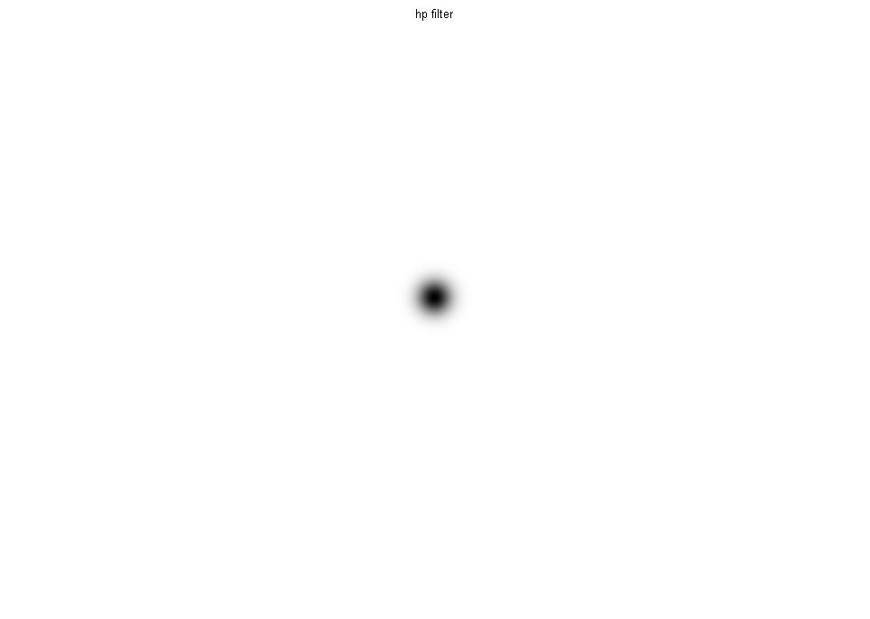
In filling the masks, we can choose to use straight up ones or zeros, to turn on or off completely any given spatial frequency component. Or, we can use any number between 0 and 1 to choose how much of a given spatial frequency component to use. In the case of using a chosen amount of a frequency, I like to use a gaussian filter with a maximum of one and approaching a minimum of zero.
My Gaussian mask making function:
I can use that function to create my gaussian type filters.
This creates filters that look like the following:
High Pass Filter from Gaussian
Low Pass Filter from Gaussian
Region Pass Filter from Gaussian
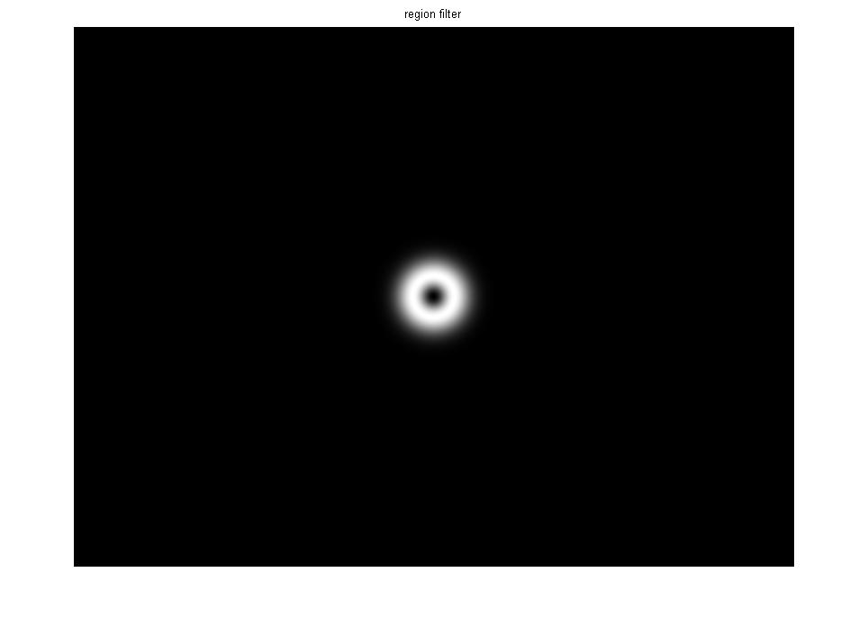
Application of these filters is shown this way:
Applying the gaussian filters:
With these filtered fourier transforms we can recontruct the image:
And, now, show them off.
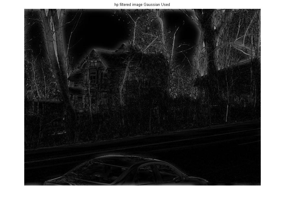

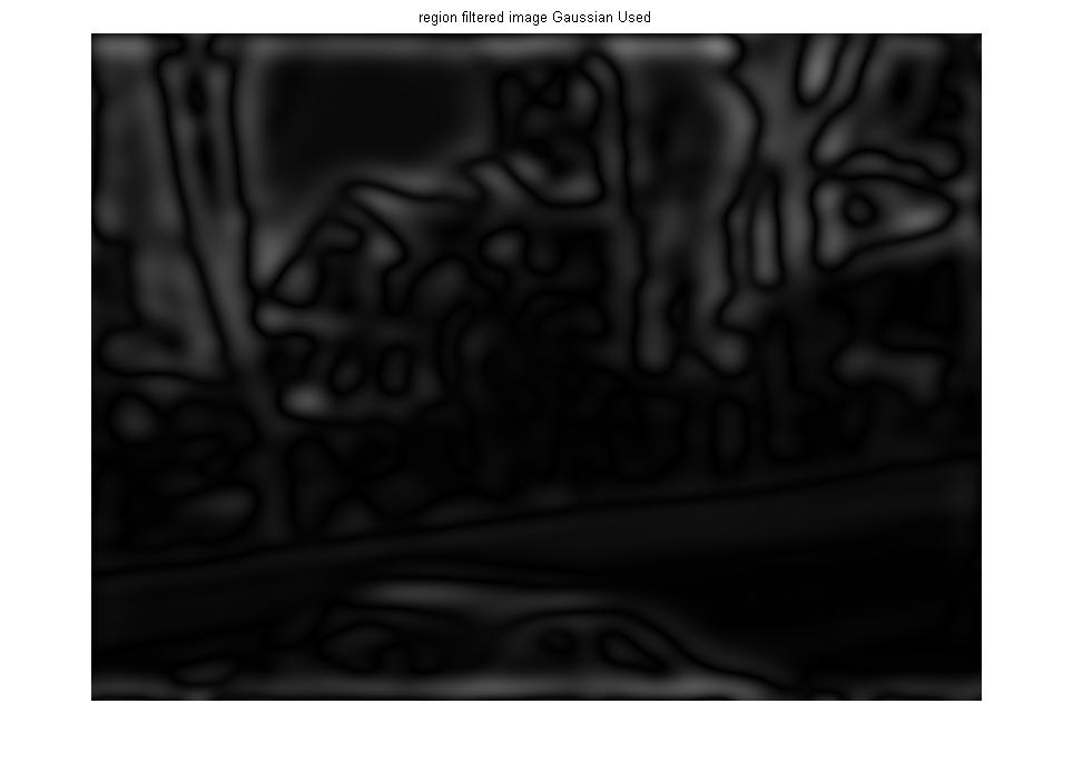
Results are a little different if use the simple on-or-off filters.
High Pass Filter on/off

Low Pass Filter on/off
Region Pass Filter on/off
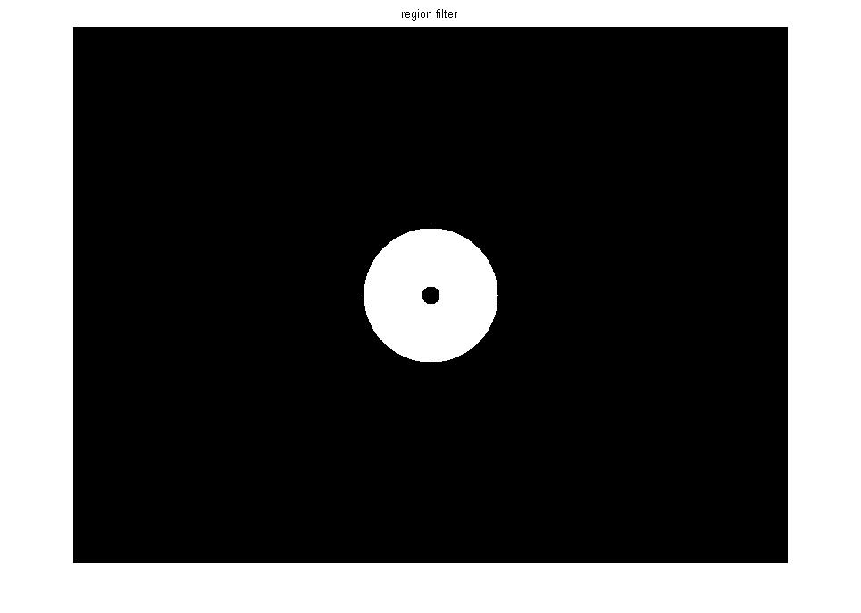
Application of these filters is shown this way:
Applying the on/off filters:
With these filtered fourier transforms we can recontruct the image:
And, now, show them off.


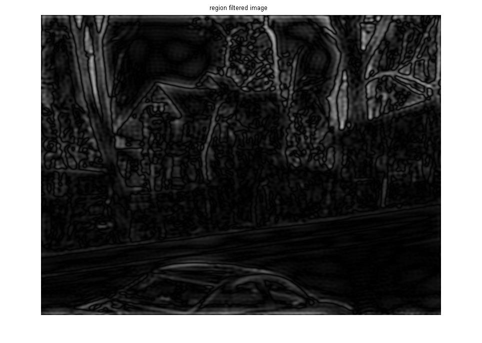
That was my quick show of how to use the DFT for image processing, using matlab in particular. I'll end this article by showing the results of a gaussian filter applied to the magnitude of an fft before recontructing the image using an image from my windows OS background options.

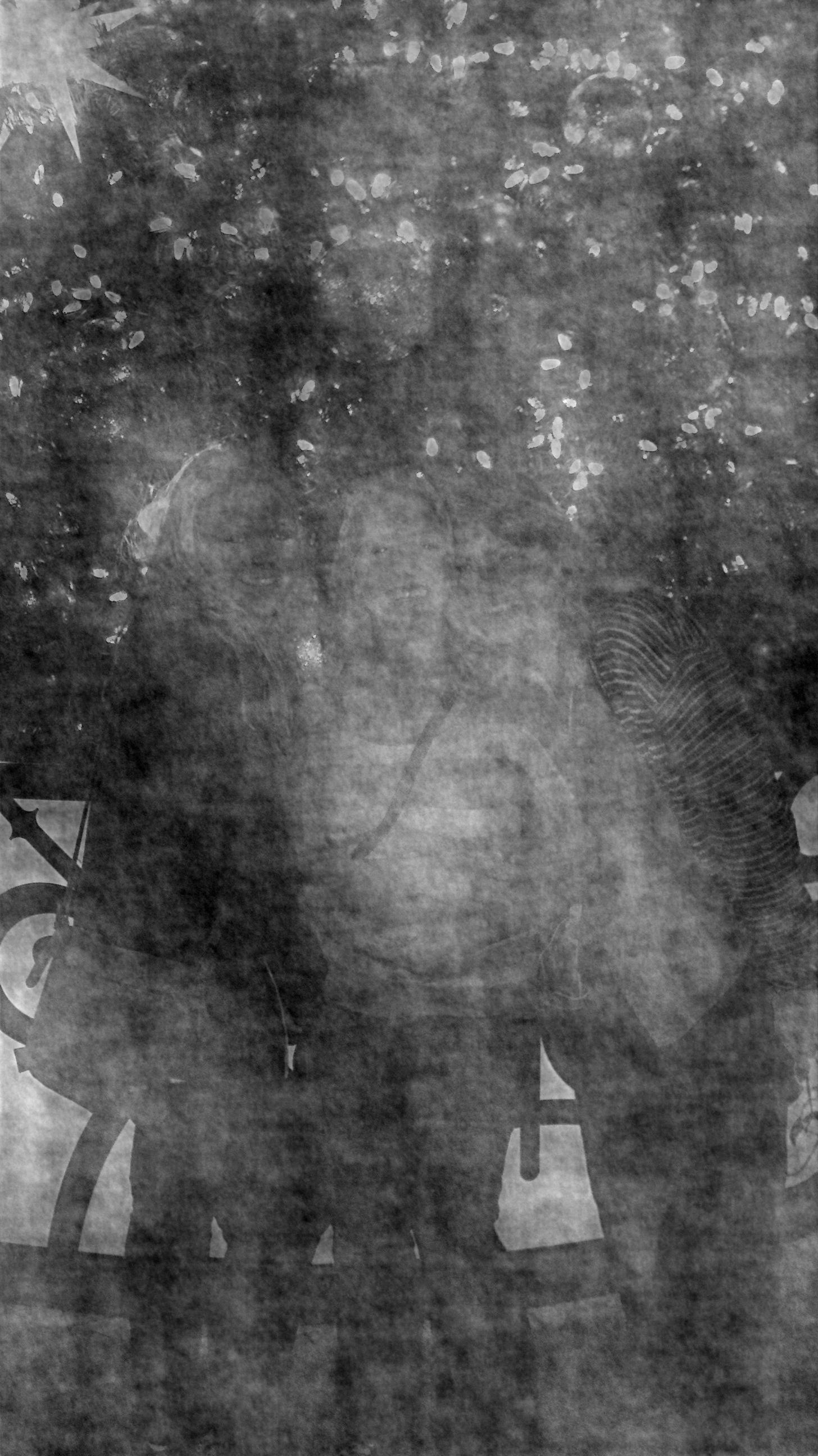
Now, I want to do something totally nonsensical. Instead of doing any filtering, I want to use the phase from my xmas girls picture:

Changed to gray scale:

with the magnitude information from my garden path picture:

Changed to gray scale:

The result looks like a strange filtered version of the one we used the phase information for!
Quick Science & Math References
- Our Solar System.
- Earth Facts.
- The Metric System.
- Trigonometric Identities.
- Vector & Tensor Identities.
- Explicit Forms of Vector Operators
- Light & Electromagnetic Spectrum.
- Common Laser Wavelengths.
- Human Physiology Facts.
- Human History Timeline
- Geologic Timeline
- Cambrian Explosion
- Life on Earth Timeline
- ASCII Codes and HTML Display Codes
- Thousands of HTML Symbol Codes
- HTML Symbol Codes for Greek Letters
- The Best Way to put Equations on your Web Page
Physics Basics Series
- Basics of Classical Mechanics.
- Basics of Quantum Mechanics.
- Basics of Electrodynamics.
- Basics of Optics.
- Basics of Mathematical Tools for Physics.
- Basics of Plasma Physics.
- Basics of Solid State Physics.
Math Basics Series
- Numbers
- Arithmetic
- Algebra
- Geometry
- Analysis
Technology Basics Series
- Basics of Remote Sensing.
- Basics of Digital Signal Processing.
- Critical Electronic Circuits
- Infrared Imaging Basics
Knowledge Branches
- Information Theory
- How Reading Works in the Brain
- Psychology of Learning
- Logic
WORK IN PROGRESS
- What is the Stark Effect?
- The Chemistry of Love &/or Addiction
- Critical Thinking: How to question what you see, read or hear.
- Aristotle's Prior Analytics - the birth of Logic.
- Optical Solutions, lenses that solve problems
- Fractals
- PTC - Photon Transfer Curve or Mean Variance Analysis
- 3-D Noise
- Laser Primer
- Rail Guns
- Special Relativity
- Radar Technology
- Acousto-optic Cells
- Harmonic Generation for Laser Frequency Doubling (SHG) and Tripling -using non-linear crystals.
- Measurement: Accuracy & Precision.
- Things you should know about computer modeling of physical phenomena!
- Giant Magneto-resistance
- Peltier Cooling
- Pyro-Electric Detectors
- Piezo-Electric Crystals
- Laser Speckle
- FFT and DFT the fast fourier transform and the discrete fourier transform
- Fabry Perot Etalon
- The Hydrogen Atom.
- PCA (Principal Component Analysis)
- Energy per mass in fuels such as Hydrogen, Gasoline, Kerosene, HMX etc...
- Nobel prize winning work on the CCD
- How does a CCD work and what are the normal characteristics of a CCD
- Nobel Prize Winning work on Giant Magneto-resistance
- FROG -frequency resolved optical gating
- Optical Wavefront Sensing
- THz imaging and time-domain spectroscopy
- Camera Calibration
- Laser Designators
- Resampling
